3.4 Combining Both Models
Combining both models is simply done by adding the finite domain model without distribution to the linear programming model. The propagator {RI.intBounds F I} is used to connect real-interval constraints with finite domain constraints. It constrains F and I to denote the same integer either as float or as integer, respectively.
declare
fun {KnapsackFDLP Problem}
   NumProducts = {Length Problem.profit}
   Resources   = Problem.resources
in
   proc {$ Sol}
      sol(maxprofit: FDMaxProfit = {FD.decl}
          products: FDProducts = {FD.list NumProducts 0#FD.sup})
      = Sol

      ObjFn Constraints
      MaxProfit = {RI.var.decl}
      Products  = {MakeList NumProducts}
   in
      %
      % finite domain constraints part
      %
      FDMaxProfit = {FD.sumC Problem.profit FDProducts '=:'}

      {ForAll {Arity Resources}
       proc {$ ResourceName}
          Resource = Resources.ResourceName
       in
          {FD.sumC Resource.npp FDProducts '=<:' Resource.ta}
       end}

      %%
      %% linear programming part
      %%
      {ForAll Products
       proc {$ V} {RI.var.bounds 0.0 RI.sup V} end}

      ObjFn = objfn(row: {Map Problem.profit {IntToFloat I}}
                    opt: max)

      Constraints =
      {Map {Arity Resources}
        fun {$ ResourceName}
          Resource = Resources.ResourceName
       in
          constr(row: {Map Resource.npp IntToFloat}
                 type: '=<'
                 rhs: {IntToFloat Resource.ta})
       end}

      %%
      %% connecting both constraint systems
      %%
      {RI.intBounds MaxProfit FDMaxProfit}
      {Map Products
       proc {$ R D} {RI.intBounds R D} end FDProducts}


      {DistributeKnapSackLP Products ObjFn Constraints
       MaxProfit}
   end
end
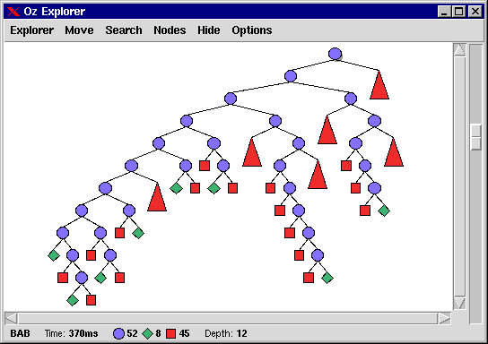
The Oz Explorer produces the following search tree by calling
{ExploreBest {KnapsackFDLP Problem}
             proc {$ O N} O.maxprofit <: N.maxprofit end}
.
